Project Part 2

Interactive and static plots of CO2 emissions from 1900 to 2019.

1. Packages I will use to read in and plot the data

library(tidyverse)
library(echarts4r)

2. Loading the data from part 1 of the project

times <- read_csv(here::here("_posts/2022-05-10-project-part-1/TIME_USE_1005.csv"))

Take a glimpse at the data

glimpse(times)

Rows: 494
Columns: 13
$ LOCATION     <chr> "AUS", "AUS", "AUS", "AUT", "AUT", "AUT", "BEL"…
$ Country      <chr> "Australia", "Australia", "Australia", "Austria…
$ DESC         <chr> "UPW", "UPW", "UPW", "UPW", "UPW", "UPW", "UPW"…
$ Description  <chr> "Unpaid work", "Unpaid work", "Unpaid work", "U…
$ SEX          <chr> "TOTAL", "WOMEN", "MEN", "TOTAL", "WOMEN", "MEN…
$ Sex          <chr> "Total", "Women", "Men", "Total", "Women", "Men…
$ AGE          <chr> "15_64", "15_64", "15_64", "15_64", "15_64", "1…
$ Age          <chr> "15-64", "15-64", "15-64", "15-64", "15-64", "1…
$ T            <chr> "LY", "LY", "LY", "LY", "LY", "LY", "LY", "LY",…
$ Time         <chr> "Latest year", "Latest year", "Latest year", "L…
$ Value        <dbl> 243.1689, 311.0000, 171.5958, 202.0000, 269.172…
$ `Flag Codes` <chr> "D", "D", "D", NA, NA, NA, NA, NA, NA, NA, NA, …
$ Flags        <chr> "Difference in methodology", "Difference in met…

3. Create an Interactive Plot

• I Start with the time data, Rename and select only needed columns
• Use group by to group Country name for each location
• Use e_chart to create an object with Value on the x axis
• Use e_river to to build lines that contain Value by each country.
• Use e_title to add title, sublink.
• Use e_theme to change theme to wonderland

times2 <- times %>%
  rename(Gender = SEX) %>%
  select(LOCATION, Country, DESC, Description, Gender, Age, T, Time, Value, `Flag Codes`, Flags)

times2 %>%
  group_by(Country) %>%
  e_chart(x = Value) %>%
  e_river(serie = Gender, legend = FALSE) %>%
  e_title(text = "Time spend base on gender and age",
          sublink = "https://ourworldindata.org/time-use",
          left = "center") %>%
  e_theme("wonderland")

4. Create Static Plot

• I start with the times2 data
• I use ggplot to create graphic object. I use Value for x and Gender for y value.
• I Geom_boxplot to demonstrate the different of time spend between gender
• I use theme_classic() to set the theme
• I use theme(legend.position= “bottom”) to set the legend at the bottom.
• I use labs to set the axis label.

times2 %>%
  ggplot(aes(x = Value, y = Gender)) +
  geom_boxplot()  + 
  theme_classic() +
  theme(legend.position = "bottom")+
  labs(y = "Gender")

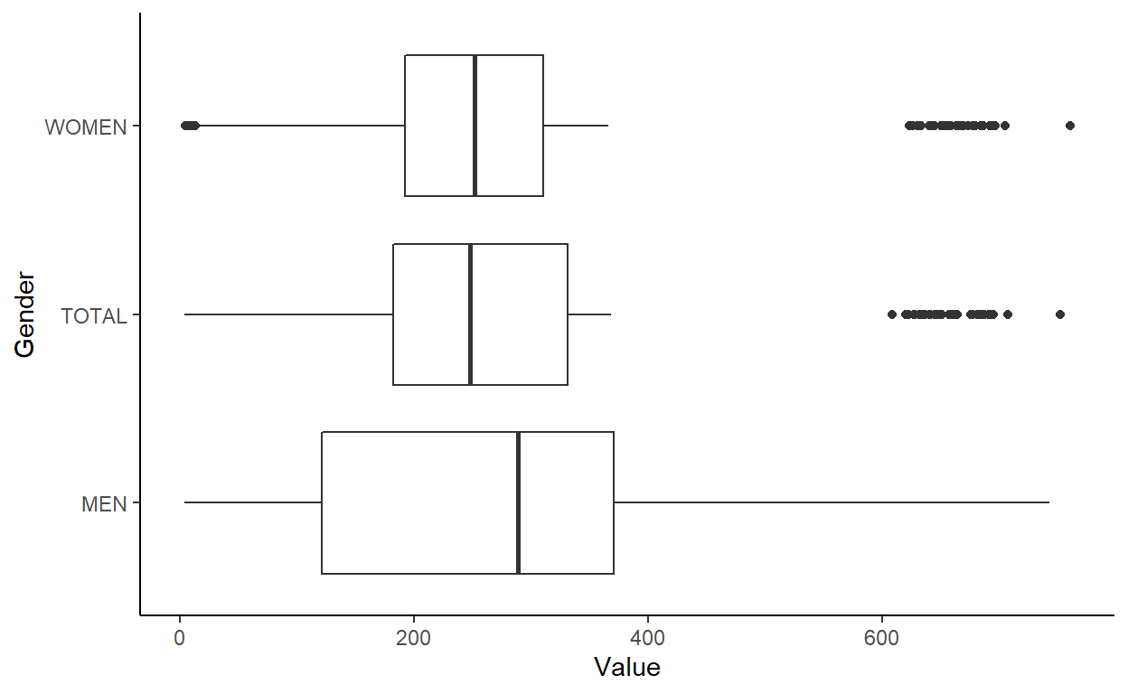
5. Describe the plot

• Men, on average, spend more leisure time than women.
• Women’s time spend have a wider spread compare to men.

6. ggsave

ggsave(filename = here::here("_posts/2022-05-17-project-part-2/preview.png"))

`